
Mid Point Rule Calculator
Mid Point Rule Calculator
Approximate a definite integral with the midpoint rule — free, in your browser, nothing uploaded. This is a numeric method: the interval is split into subintervals, the function is evaluated at each midpoint, and those values are summed and multiplied by the subinterval width. The full table of midpoints and values is shown, so every step can be checked.
Use x, numbers, + – * / ^, brackets, and sin, cos, tan, exp, log, sqrt, abs, pi, e.
Some integrals refuse to be integrated. Functions like e^(−x²) or sin(x)/x have no antiderivative in terms of the familiar functions, yet their definite integrals have perfectly definite values that physics, statistics, and engineering need as numbers. That is why numeric integration exists: a family of methods that approximate the area under a curve by adding up simple shapes. The midpoint rule is the friendliest of them. Slice the interval into n equal subintervals, evaluate the function once at the centre — the midpoint — of each slice, treat that height as a rectangle spanning the slice, and add the rectangles. A mid point rule calculator does exactly this and shows its working: enter a function, the limits a and b, and the number of subintervals n, and the calculator at the top of this page prints the width, every midpoint, every function value, the sum, and the final approximation, so not one step hides inside the machine.
The midpoint rule earns its popularity with a small miracle of balance. On any single subinterval, using the midpoint's height overestimates the area on one side of the centre and underestimates it on the other, and for a smooth curve those two errors partly cancel. The result is that the midpoint rule is roughly twice as accurate as the more obvious left-endpoint or right-endpoint rectangle rules with the same number of slices, and it matches the trapezoidal rule's error order while often beating its constant. It is an approximation — it does not pretend otherwise, and this tool labels its output numeric and states how to improve it — but it is a principled one, and with enough subintervals it will take you as close to the true integral as you have patience for.
What It Is
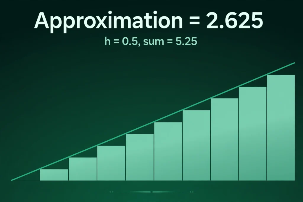
The definite integral of f(x) from a to b is the signed area between the curve and the x-axis: area above the axis counts positive, area below counts negative. The midpoint rule approximates that area with n rectangles of equal width h = (b − a)/n. The i-th rectangle stands over the i-th subinterval, and its height is the function's value at the subinterval's midpoint, x = a + (i + 0.5)h. The approximation is M = h × [ f(midpoint 1) + f(midpoint 2) + … + f(midpoint n) ]. Everything in the method is inside that one line, and the calculator's steps are just that line computed openly: h first, then a table of midpoints and values, then the sum, then the multiplication.
Two properties are worth knowing before you trust any output. First, accuracy: for a smooth function, the midpoint error shrinks roughly like 1/n², so doubling the subintervals quarters the error, and computing with n and then 2n and watching the change is a practical accuracy check — when the two answers agree to the digits you need, you have your number. Second, exactness in a special case: for a straight-line function, the midpoint rule is exact for any n, even n = 1, because the over- and under-estimates on either side of the centre cancel perfectly for a line. For curves, the cancellation is partial, improving as the slices narrow and each slice looks more like a line. The tool caps n at 200, not because the method fails beyond that, but because its promise is to show you the full table of midpoints and values, and a table you cannot read is a step you cannot check.
How to Use the Calculator
Using the tool takes less than a minute. Follow these steps:
- Enter the function f(x) using x, numbers, + - * / ^, brackets, and sin, cos, tan, exp, log, sqrt, abs, pi, e. The live test uses x^2. Note that log means the natural logarithm, and trig functions take radians.
- Enter the lower limit a and the upper limit b. The live test uses a = 0 and b = 2.
- Enter the number of subintervals n, a whole number from 1 to 200. The live test uses n = 4.
- Press "Calculate Midpoint Approximation" and read the width h, the table of midpoints and function values, the sum of the values, and the final result h × sum.
- For an accuracy check, run again with double the n and compare: the change between the two results is a fair guide to the remaining error.
If the function is undefined or infinite at any midpoint — for example, 1/x across an interval containing 0 — the tool stops and tells you which midpoint failed, rather than printing a meaningless total. Singularities inside an interval need specialised methods, and the limits section says more about that.
How does the midpoint rule compare with the left, right, trapezoidal, and Simpson rules?
| Method | Sample point in each slice | Error order for smooth functions | Notes |
| left endpoint | left end | about 1/n | crudest rectangle rule |
| right endpoint | right end | about 1/n | same order as left |
| midpoint | centre | about 1/n^2 | one evaluation per slice, no endpoint values needed |
| trapezoidal | average of both ends | about 1/n^2 | roughly twice the midpoint error constant, opposite sign |
| Simpson | parabola through three points | about 1/n^4 | needs an even number of slices and a smoother function |
Refinement table for x^2 from 0 to 2 (exact 8/3 = 2.666667):
| n | Approximation | Error |
| n=4 | 2.625 | error -0.0417 |
| n=8 | 2.65625 | error -0.0104 |
| n=16 | 2.664062 | error -0.0026 |
| n=32 | 2.666016 | error -0.0007 |
Each doubling cuts the error to about a quarter, matching the 1/n^2 order.
What input formats does this tool accept?
Write multiplication explicitly: enter 3*x+1, not 3x+1 — the function parser rejects implicit multiplication with the error 'Could not evaluate the function: Extra characters at the end of the function.' Enter limits as numbers: for sin(x) from 0 to pi, enter b as 3.14159265, not pi — the limit field rejects pi with 'Please enter a number for b.' (The function field itself accepts pi.)
Worked Examples
Example 1: x² from 0 to 2 with n = 4, the live test
Function x^2, limits 0 to 2, n = 4. Width h = (2 − 0) / 4 = 0.5. The subintervals are [0, 0.5], [0.5, 1], [1, 1.5], [1.5, 2], with midpoints 0.25, 0.75, 1.25, and 1.75. Function values: f(0.25) = 0.0625, f(0.75) = 0.5625, f(1.25) = 1.5625, f(1.75) = 3.0625. Sum = 5.25. Approximation = h × sum = 0.5 × 5.25 = 2.625. The exact integral of x² from 0 to 2 is 8/3 ≈ 2.6667, so with only four rectangles the midpoint rule is within about 0.04 — roughly 1.6 percent low, because the curve bends upward and each midpoint rectangle slightly under-fills the slice. Double to n = 8 and the approximation becomes about 2.6563, cutting the error to about 0.01, consistent with the quartering pattern the theory predicts.
Example 2: A line, where the rule is exact — 3*x + 1 from 0 to 4 with n = 2
Function 3*x + 1, limits 0 to 4, n = 2. Width h = 2. Midpoints: 1 and 3. Values: f(1) = 4, f(3) = 10. Sum = 14. Approximation = 2 × 14 = 28. The exact integral is [1.5x² + x] from 0 to 4 = 24 + 4 = 28. Exact, with just two rectangles, exactly as promised for linear functions. If your function is a line — a rate that changes at a constant rate, a cost that grows steadily — the midpoint rule is not an approximation at all, and seeing one exact case builds the right intuition for why nearly straight slices behave nearly exactly.
Example 3: A curve with no simple antiderivative habit — sin(x) from 0 to π with n = 4
Function sin(x), limits 0 to 3.14159265 (enter the number for the limit; the function field itself accepts pi), n = 4. Width h = pi/4 ≈ 0.785398. Midpoints: pi/8, 3pi/8, 5pi/8, 7pi/8, approximately 0.3927, 1.1781, 1.9635, 2.7489. Sine values: about 0.382683, 0.923880, 0.923880, 0.382683 — note the symmetry, since the sine arch is symmetric about pi/2. Sum ≈ 2.613126. Approximation ≈ 0.785398 × 2.613126 ≈ 2.0523. The exact integral is 2, so four midpoints overshoot by about 0.05; the arch bulges upward, and midpoint rectangles on a downward-bending top overestimate slightly. Same method, opposite error direction from Example 1 — the sign of the error follows the curve's bending, which is why comparing two values of n is more trustworthy than any rule of thumb about over- or under-estimates.
Example 4: Signed area — x from −1 to 2 with n = 3
Function x, limits −1 to 2, n = 3. Width h = 1. Midpoints: −0.5, 0.5, 1.5. Values: −0.5, 0.5, 1.5. Sum = 1.5. Approximation = 1.5, and since the function is linear it is exact: the exact integral is [x²/2] from −1 to 2 = 2 − 0.5 = 1.5. Notice the first midpoint contributes a negative value: on [−1, 0] the function sits below the axis, and that area counts against the total. Definite integrals are signed areas, and the midpoint rule inherits the convention automatically — no special handling is needed, but you must remember it when an answer comes out smaller than the geometric area you pictured, or even zero for a function balanced above and below the axis.
There is also a practical reason the midpoint rule is the default in much scientific software: it never asks for the function's values at the interval's endpoints. Endpoint values are exactly where real-world functions misbehave — a measurement that starts at zero velocity, a density that spikes at a boundary, a formula with a removable glitch at a = 0. Sampling only interior midpoints sidesteps those trouble spots while losing nothing in accuracy order. If your function is awkward precisely at an endpoint but smooth inside, the midpoint rule is not merely convenient; it may be the only one of the simple rules that runs at all, and this calculator's table shows every sampled point so you can confirm they are all interior.
Midpoint Rule Versus Its Neighbours
Three sibling methods slice the same interval. The trapezoidal rule joins the function's values at the slice endpoints with straight lines and averages left and right endpoints; its error is the same order as the midpoint rule's, with roughly twice the constant and the opposite sign on smooth curves — averaging a midpoint and a trapezoidal result cancels much of both errors, a trick behind more advanced schemes. Simpson's rule fits parabolas through triples of points and is a step up in accuracy order, at the cost of requiring an even number of subintervals and a smoother function. The endpoint rectangle rules (left or right sums) are a full order cruder. The midpoint rule's charm is the ratio of simplicity to accuracy: one evaluation per slice, no endpoint bookkeeping, and an error that behaves predictably under refinement. When you need a quick, defensible number and intend to show your working, it is hard to beat. When you need six guaranteed decimals, refine n until the answer stabilises, or move up to Simpson's rule with the same doubling discipline.
Common Mistakes
The first common mistake is using endpoints instead of midpoints — evaluating at a, a + h, and so on, which is a different (and weaker) rule; the calculator's table exists partly so you can confirm each evaluation point really is a centre, a + (i + 0.5)h. The second mistake is entering degrees into trig functions: this tool's sin and cos take radians, so sin(x) from 0 to 180 is not the arch you want; use 0 to pi. The third mistake is treating the first approximation as the answer: one run with a small n is a sketch, and the honest workflow is to double n and compare. The fourth mistake is integrating blindly across a singularity — 1/x from −1 to 1 has no ordinary definite integral value at all, and a numeric sum that returns a tidy number there is lying to you; the tool stops when a midpoint itself is undefined, but a singularity between midpoints can still corrupt a result, so inspect your function for blow-ups before integrating. The fifth mistake is forgetting that the result is signed area: a negative or zero approximation may be correct behaviour, not a bug.
Limits: What This Tool Does and Does Not Do
This tool computes the midpoint rule approximation to a definite integral of a function you enter, with n from 1 to 200 subintervals, showing the width, every midpoint, every function value, the sum, and the product. It is a numeric approximation, not an exact antiderivative: it cannot return a formula, and its number differs from the true integral by an error that shrinks as n grows for smooth functions. The function is read by a safe parser written for this tool — no eval — supporting + - * / ^, brackets, sin, cos, tan, exp, log (natural), sqrt, abs, pi, and e; anything else is rejected with an error message. Angles are in radians. If the function is undefined or infinite at a midpoint, the tool stops and names the midpoint. It does not detect singularities hiding between midpoints, does not split intervals at discontinuities for you, and does not do improper integrals to infinity. Within those limits, every line of its table is the real computation.
Privacy: Your Numbers Stay in Your Browser
Every function and limit you enter into this mid point rule calculator stays in your browser. Nothing is uploaded to a server, nothing is stored, and there is no account to create. The calculation runs entirely on your own device, and closing the page removes your inputs. This browser-only design is the same principle behind the other free tools on Your Smart Kit: a simple tool that does one job well, keeps your data private, and gives an answer you can check.
Frequently Asked Questions
What is the midpoint rule formula?
M = h × [ f(x1*) + f(x2*) + … + f(xn*) ], where h = (b − a)/n is the subinterval width and each xi* is a subinterval's midpoint, a + (i − 0.5)h. The calculator prints h, every midpoint, every value, and the sum, so the formula is computed in the open.
How accurate is the midpoint rule?
For smooth functions the error falls roughly like 1/n²: doubling n quarters the error. In the live test, n = 4 gives 2.625 against the exact 2.6667, and n = 8 gives about 2.6563. The practical accuracy test is to double n and watch how much the answer moves.
How many subintervals should I use?
Enough that doubling n stops changing the digits you care about. Start with n = 10 or 20, double once, and compare. Very wiggly functions need more; straight lines need only n = 1, since the rule is exact for them.
Why does the calculator cap n at 200?
Because it shows the full table of midpoints and values as checkable steps, and a table longer than 200 rows cannot be read. If you need more refinement, the pattern from two smaller runs — the change shrinking by about a factor of four per doubling — tells you where the answer is heading.
What does the calculator do with area below the axis?
It counts it as negative, as definite integrals do. Values at midpoints below the axis enter the sum with their sign, so the result is the signed (net) area. For total geometric area, split the interval at the zeros of the function and add the absolute values of the pieces.
Does log mean base 10 or base e here?
Base e — the natural logarithm, matching the mathematical convention in calculus. The parser also accepts ln as the same function. If you need log base 10, use log(x)/log(10).
Related Tools on Your Smart Kit
If you found the mid point rule calculator useful, you may also like the other free calculators on Your Smart Kit, including the piecewise integral calculator for integrating functions defined in pieces, the infinite series calculator with steps for watching partial sums settle, and the partial differentiation calculator for rates of change of two-variable functions. Each runs in your browser, free, with no sign-up, and each is built on the same principle: a simple tool that does one job well, keeps your data private, and gives an answer you can check. Try the mid point rule calculator at the top of this page with your own function, then double n and watch the approximation tighten.