Population Growth Calculator

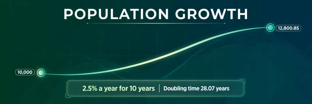
A town of 10,000 people growing at 2.5% a year does not gain a neat 250 people annually and stop there. It gains 250 the first year, then 256, then 263 — the increase itself increases, because each year’s growth is calculated on a larger population than the year before. After ten years the town holds 12,800.85 people, not the 12,500 a straight-line guess would give. A population growth calculator applies that compounding properly: give it a starting population, an annual growth rate, and a number of years, and it returns the final population, the total increase, and a year-by-year table so you can watch the compounding happen rather than take it on trust.

The model underneath is the same exponential growth that governs compound interest, bacteria in a dish, and the early spread of a rumour — anything whose growth in each period is a fixed proportion of its current size. That is both the model’s strength and its limitation. It is the right first approximation for populations over short and medium horizons, for classroom problems, for planning estimates, and for understanding why demographers talk in rates rather than absolute numbers. It is not a crystal ball: real populations change their rates as cities fill, economies shift, and people move. A good calculator says that plainly, shows its steps, and lets you test other rates quickly — which is what the tool at the top of this page is built to do.

What Population Growth Means

A population’s growth rate bundles together everything that changes its size: births add, deaths subtract, immigration adds, emigration subtracts. Demographers usually quote the net result as a percentage per year. A rate of 2.5% means that, all effects combined, the population at the end of a year is 1.025 times the population at the start. Apply that multiplier repeatedly and you have the model:

Final population = P0 × (1 + r/100)^t

where P0 is the initial population, r is the annual growth rate in percent, and t is the number of years. The quantity (1 + r/100) is the annual growth factor — the single most useful number in the output, because it converts the percentage language of reports into the multiplication the population actually experiences. A growth factor of 1.025, applied ten times, is 1.025^10 ≈ 1.280085, which is why the live test’s 10,000 becomes 12,800.85: a total increase of 2,800.85, or 28.01% overall. Notice that 28.01% is more than ten times 2.5% — the extra 3.01 percentage points are the compounding, growth earned on earlier growth, exactly as interest earns interest in a savings account.

Negative rates fit the same formula without any special casing. A rate of −2% gives a growth factor of 0.98, and each year the population keeps 98% of itself: 5,000 declining at 2% a year for five years becomes 5,000 × 0.98^5 = 4,519.60, a total fall of 480.40, or −9.61% overall — less than five times 2%, because a shrinking population loses fewer people each year in absolute terms. This symmetry is worth internalising: constant-percentage change always curves, up or down, and the curve is what the year-by-year table in the tool makes visible.

Two derived ideas complete the picture. The doubling time — how long a growing population takes to double — depends only on the rate: at 2.5% it is about 28 years (the rule of 70 gives 70 / 2.5 = 28, and the exact figure is ln 2 / ln 1.025 ≈ 28.07). And the distinction between this exponential model and a logistic model matters for long horizons: logistic growth bends the curve as a population approaches a carrying capacity, while the exponential model in this tool keeps compounding at the stated rate forever. Over ten or twenty years the two are often close; over two hundred, they are not, and the limits section below is honest about that.

How to Use the Calculator

Using the tool takes a few seconds. Follow these steps:

1. Enter the initial population, P0. The live test uses 10,000. It can be a town, a country, a herd, a colony of bacteria — anything counted in individuals.
2. Enter the annual growth rate as a percent. The live test uses 2.5. Use a negative number for decline; the tool accepts rates down to −100.
3. Enter the number of whole years. The live test uses 10. Years are whole numbers because the table grows the population one full year at a time; the tool accepts up to 500.
4. Press “Calculate Population Growth”.
5. Read the final population, the total increase and overall percentage, then scan the year-by-year table to see the compounding year by year.

The table is capped at the first 25 rows (years 0 to 25) so the page stays readable; when you ask for more years, the tool says so and still computes the final figure for the full span.

Worked Examples

Example 1: The live test — 10,000 at 2.5% for 10 years

Enter P0 = 10,000, r = 2.5, t = 10. The tool returns a final population of 12,800.85 and a total increase of 2,800.85 (28.01% overall), with growth factor 1.025. The table shows the curve forming: year 0: 10,000.00; year 1: 10,250.00; year 2: 10,506.25; year 3: 10,768.91; year 4: 11,038.13; year 5: 11,314.08; year 6: 11,596.93; year 7: 11,886.86; year 8: 12,184.03; year 9: 12,488.63; year 10: 12,800.85. Compare the yearly increments: the first year adds 250.00, the tenth adds 312.22. Same rate, bigger base, bigger step. Any projection that adds a constant number per year understates a growing population and overstates a shrinking one — this table is the antidote.

Example 2: A declining population

A village of 5,000 is losing people at 2% a year. Enter P0 = 5,000, r = −2, t = 5. The final population is 4,519.60, a total increase of −480.40 (−9.61% overall). The negative increase is the honest way to present a fall. Village planners use exactly this projection, run further out, to decide whether a school or a clinic stays viable; the model’s message here is that the decline slows in absolute terms even at a constant rate, because 2% of a smaller village is fewer people leaving.

Example 3: A fast-growing city

A city of 800,000 grows at 4.5% a year — a brisk rate that some fast-urbanising cities genuinely post. Enter P0 = 800,000, r = 4.5, t = 10. The final population is 1,242,365.30, a total increase of 442,365.30 (55.30% overall). That is more than 400,000 extra people in a decade — the equivalent of a whole new city inside the city, with housing, water, transport and schools to match. The tool’s lesson is plain: rates that sound modest compound into city-scale change, and the table’s last rows, where each year adds nearly 50,000 people, show why infrastructure built for the first year’s growth will fall behind by year ten.

Example 4: Bacteria, where the rate is huge

A culture of 1,000 cells doubles every 20 minutes, which is an hourly rate of 700% — the growth factor per hour is 8, since three doublings multiply by 2 × 2 × 2. The tool’s inputs are annual rates, so a laboratory example is cleaner as a thought experiment: 1,000 cells at 100% a year for 3 years gives 8,000. Enter P0 = 1,000, r = 100, t = 3: the final population is 8,000.00, a total increase of 7,000.00 (700.00% overall), growth factor 2. This is why microbiology runs in hours rather than years: at these rates the model hits absurd numbers within a day, which is also why it stops being realistic — the dish runs out of food, and logistic growth takes over. The calculator stays honest at any rate you enter; you supply the judgement.

How to Read the Output

The headline result is the final population after the number of years you entered, written with two decimal places. Beneath it, the total increase is the final population minus the starting population, shown as a signed number, and the overall percentage is that increase divided by the starting population, multiplied by 100. The growth factor per year is 1 + r/100, the multiplier applied every year. The step lines show the chain: growth factor, then the raising to the power of years, then the multiplication that gives the final population. The table gives the population at the end of each year, starting at year 0 — the starting population, unchanged — and ending at the year you entered, or at year 25 when you entered more than that. If the output does not look like the example above, check that you typed the rate as a percent (2.5, not 0.025) and that years is a whole number.

Where Population Growth Projection Is Used

Town planners project school rolls, water demand and bus routes from population growth. Health officials project vaccine doses and hospital beds. Ecologists project an invasive species’ spread before it reaches a new habitat, and fisheries managers project a stock’s recovery under a catch limit. Businesses project a customer base, or a market, growing at a steady rate — the mathematics is identical, and the tool’s population label is only a label; P0 can be customers, subscribers, or trees. Historians and demographers use the same model in reverse, asking what constant rate connects a census figure in 1950 to one in 2000. And teachers use it as the cleanest introduction to exponential growth, because a population doubling is the most vivid example of a curve that outruns every straight line drawn from it.

A Note on Sensitivity: Small Rate Differences, Large Outcomes

Run the live test twice, once at 2.0% and once at 3.0%, and the ten-year results differ by more than a thousand people: 12,189.94 versus 13,439.16 on a base of 10,000. A single percentage point of rate is worth over 12% of the starting population after a decade, because it compounds. Run it over fifty years and the gap is enormous: 26,915.83 at 2% versus 43,839.29 at 3%. This is the single most important practical lesson of the tool. Population forecasts are only as good as their rates, and rates are the hardest part to estimate — births, deaths and migration all move with policy, economics and events. Always run a range: a low, a central and a high rate, and present the spread as honestly as the central figure.

Common Mistakes

The most common mistake is typing the rate as a decimal: 0.025 instead of 2.5. The tool would then grow the population at 0.025% a year and return 10,025.03 after ten years — a result that looks plausible enough to miss, so check the growth factor in the steps: it should be 1.025, not 1.00025. The next mistake is treating the growth factor as the rate: entering 1.025 as the rate means 1.025% a year, not 2.5%. A third is entering a fractional number of years and expecting the table to show part-years; the tool uses whole years, so a 10.5-year horizon is approximated by 10 or 11. Finally, people apply the constant-rate model to populations they know are saturating — a town bounded by green belt, an island fishery, a market approaching saturation — and are surprised when the projection overshoots. That is the model’s assumption talking, not its arithmetic.

Limits: What This Tool Does and Does Not Do

The tool projects at one constant rate. Real populations rarely oblige: fertility falls as countries develop, migration surges after wars and policy changes, pandemics and famines interrupt the curve. The tool does not model age structure — a population with many young people will keep growing even at replacement fertility, a momentum the simple model cannot see. It does not model carrying capacity, so it will happily project a town past its water supply. And its results are not whole people: 12,800.85 is a statistical expectation, not a headcount, and the two decimals are there for checking arithmetic, not for claiming that precision about the future. For official forecasts, use cohort-component models from a national statistics office; for understanding, planning ranges and homework, this tool is the right weight.

Privacy: Your Numbers Stay in Your Browser

Like every tool on Your Smart Kit, this calculator runs entirely in your browser. Your starting population, rate and years are never sent to a server, stored, or shared — there is no account, no tracking of inputs, and nothing to delete afterwards. You can use it for sensitive planning figures, such as a business’s customer base or a hospital’s catchment, with the same confidence as a pocket calculator.

Frequently Asked Questions

What is the population growth formula?

Final population = P0 × (1 + r/100)^t, where P0 is the starting population, r is the annual growth rate in percent, and t is the number of years. The tool shows each step so you can follow the arithmetic.

What is the difference between growth rate and growth factor?

The growth rate is the percentage, such as 2.5%. The growth factor is 1 + r/100 — 1.025 for a 2.5% rate — the number the population is multiplied by each year. The tool reports both, because reports quote rates and calculations use factors.

Can the growth rate be negative?

Yes. A negative rate models a declining population: the growth factor falls below 1, and each year keeps that fraction of the previous year. Enter −2 for a population shrinking at 2% a year.

Why is the total percentage more than rate × years?

Because growth compounds: each year’s increase is calculated on a larger population, so the increases themselves grow. Ten years at 2.5% gives 28.01% overall, not 25% — the extra 3.01 percentage points are growth on earlier growth.

Why is the table capped at 25 rows?

So the page stays readable. The tool shows years 0 to 25 and always computes the final figure for the full number of years you entered, up to 500, even when the table stops early.

Is a population of 12,800.85 people realistic?

As a headcount, no — populations are whole people. The decimals are a statistical expectation and an arithmetic check: they let you verify the calculation and compare scenarios precisely, then round to whole people for any real-world use.

Related Tools on Your Smart Kit

If you found this calculator useful, you may also like the Cost Index Calculator, which adjusts an amount between two dates using index values, and the Present Value of Money Calculator, which discounts a future amount to today’s value, and the Compound Interest Calculator, which grows a sum at a steady rate — all three use the same compounding idea in different clothes, and all three run entirely in your browser.

Doubling time at every rate: exact figures against the rule of 70

Doubling time depends only on the rate. The exact figure is ln 2 / ln(1 + r/100); the rule of 70 (70 / rate) is a shortcut. The 10-year populations below are live tests on this page; doubling times are computed from the verified formula.

Annual rate	Population after 10 years, from 10,000	Exact doubling time	Rule of 70
1%	11,046.22	69.66 years	70.0 years
2%	12,189.94	35.00 years	35.0 years
2.5%	12,800.85	28.07 years	28.0 years
3%	13,439.16	23.45 years	23.3 years
5%	16,288.95	14.21 years	14.0 years

The rule of 70 is within a fraction of a year at rates up to 3%, and still within a quarter of a year at 5% — close enough for a quick estimate, but use the exact figure when the doubling time itself is the answer you need. Read the table the other way too: a single percentage point (2% to 3%) is worth 1,249.22 extra people after ten years on a base of 10,000.