SE Calculator
Paste a list of numbers, or enter a mean, a standard deviation and a sample size, and the tool works out the standard error and the 95% confidence interval.
Separate the numbers with commas, spaces or line breaks.
The 95% interval uses the normal approximation (z = 1.96). For small samples a t-interval is wider and more honest — see the section below. Your entries stay in your browser.
The standard error (SE) of a sample mean tells you how far that mean is likely to sit from the true population mean. This tool works it out two ways: paste a list of numbers and it gives you the count, mean, standard deviation, variance, standard error, margin of error and the 95% confidence interval; or enter a mean, a standard deviation and a sample size directly and it gives you the standard error, the margin of error and the 95% confidence interval.
How do I use the SE Calculator?
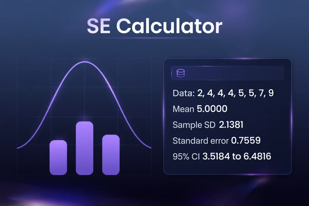
Choose a mode at the top of the tool. In “Paste a list of numbers” mode, type or paste your numbers into the box, separated by commas, spaces or line breaks — for example “2, 4, 4, 4, 5, 5, 7, 9” — and press Calculate. The tool shows ten results: the count, the sum, the mean, the sample standard deviation, the population standard deviation, the sample variance, the population variance, the standard error, the margin of error at 95%, and the 95% confidence interval. A line under the results shows the working, so you can follow each step.
In “Enter mean, SD and sample size” mode, enter the sample mean, the sample standard deviation (s) and the sample size (n), then press Calculate. This mode is for when you already have those three summary figures — from a paper, a report or another calculation — and only need the standard error and the interval. It shows the standard error, the margin of error and the 95% confidence interval, with the working underneath.
If an input is wrong, the tool shows a plain-language error and no results. A blank list is rejected with “Enter your numbers first.” A list of more than 10,000 numbers is rejected with “Enter 10,000 numbers or fewer.” A single value is rejected with “A single value has no standard deviation or standard error. Enter at least two numbers.” — because the sample standard deviation divides by n−1, and with one value that division has no answer. A token that is not a number is rejected by name, for example “The entry “abc” is not a number. Use numbers separated by commas, spaces or line breaks.” In direct-entry mode, a blank mean, standard deviation or sample size is rejected with a message naming the missing field; a negative standard deviation is rejected, because a standard deviation cannot be below 0; and a sample size below 2, or not a whole number, is rejected, because the standard error of a mean needs at least two whole observations.
What does a worked example look like?
Take the eight numbers 2, 4, 4, 4, 5, 5, 7, 9. Work through them step by step.
Step 1 — the mean. There are 8 numbers and they add up to 40, so the mean is 40 / 8 = 5.0000.
Step 2 — the deviations. Subtract the mean from each number: −3, −1, −1, −1, 0, 0, 2, 4. Square each one: 9, 1, 1, 1, 0, 0, 4, 16. Add the squares: 9 + 1 + 1 + 1 + 0 + 0 + 4 + 16 = 32.0000. That total is the sum of squared deviations.
Step 3 — the variances. The sample variance divides by n−1, which is 7: 32.0000 / 7 = 4.5714. The population variance divides by n, which is 8: 32.0000 / 8 = 4.0000.
Step 4 — the standard deviations. Take the square root of each variance. The sample standard deviation is √4.5714 = 2.1381. The population standard deviation is √4.0000 = 2.0000.
Step 5 — the standard error. Divide the sample standard deviation by the square root of the sample size: SE = 2.1381 / √8 = 2.1381 / 2.8284 = 0.7559.
Step 6 — the margin of error and the interval. Multiply the standard error by 1.96, the z-value for 95% confidence: 1.96 × 0.7559 = 1.4816. The 95% confidence interval is the mean plus or minus that margin: 5.0000 ± 1.4816, which runs from 3.5184 to 6.4816.
A second example uses a different set of numbers. Take 10, 12, 14, 16, 18. There are 5 numbers, they add up to 70, and the mean is 70 / 5 = 14.0000. The deviations are −4, −2, 0, 2, 4, and their squares are 16, 4, 0, 4, 16, which add up to 40.0000. The sample variance is 40.0000 / 4 = 10.0000, so the sample standard deviation is √10.0000 = 3.1623. The population variance is 40.0000 / 5 = 8.0000, so the population standard deviation is √8.0000 = 2.8284. The standard error is 3.1623 / √5 = 3.1623 / 2.2361 = 1.4142. The margin of error is 1.96 × 1.4142 = 2.7719, and the 95% confidence interval is 14.0000 ± 2.7719, from 11.2281 to 16.7719. All figures are rounded to four decimal places at the end, so multiplying the rounded figures by hand can differ in the last digit.
A third example uses the direct-entry mode. A study reports a mean of 50, a sample standard deviation of 10 and a sample size of 25. The standard error is 10 / √25 = 10 / 5 = 2.0000. The margin of error is 1.96 × 2.0000 = 3.9200. The 95% confidence interval is 50 ± 3.9200, from 46.0800 to 53.9200. This is the mode to use when the raw data are not available and only the summary figures are printed.
A fourth example shows what two numbers alone can do. Take 3 and 7. The mean is 5.0000, the deviations are −2 and 2, the squared deviations are 4 and 4, and the sum of squared deviations is 8.0000. The sample variance is 8.0000 / 1 = 8.0000, so the sample standard deviation is √8.0000 = 2.8284. The population variance is 8.0000 / 2 = 4.0000, so the population standard deviation is 2.0000. The standard error is 2.8284 / √2 = 2.8284 / 1.4142 = 2.0000, the margin of error is 3.9200, and the 95% confidence interval runs from 1.0800 to 8.9200. Two numbers give a very wide interval, which is the tool telling you plainly that two observations carry almost no information about the population mean.
A fifth example uses a larger, evenly spaced set: 12, 15, 18, 21, 24, 27, 30, 33, 36, 39. There are 10 numbers, they add up to 255, and the mean is 25.5000. The sum of squared deviations is 742.5000, so the sample variance is 742.5000 / 9 = 82.5000 and the sample standard deviation is 9.0830. The population standard deviation is 8.6168. The standard error is 9.0830 / √10 = 2.8723, the margin of error is 5.6297, and the 95% confidence interval runs from 19.8703 to 31.1297.
What is standard error?
The standard error of the mean is the standard deviation of the sample mean itself. Picture drawing many samples of the same size from the same population and working out the mean of each one. Those means would not all be equal: they would spread around the true population mean. The standard error is the size of that spread. A small standard error means the sample means cluster tightly around the true mean, so one sample’s mean is a good estimate. A large standard error means they scatter widely, so one sample’s mean could be a long way off.
That is the whole point of the tool. A mean on its own says nothing about how much to trust it. A mean of 50 with a standard error of 2.0000 is a precise estimate; a mean of 50 with a standard error of 20 would be almost useless. The standard error turns a bare average into a statement about precision, and the confidence interval turns it into a range of plausible values for the true mean.
The idea comes from the central limit theorem: the mean of n independent observations has a variance of σ²/n, where σ is the population standard deviation, so its standard deviation is σ/√n. Because the true σ is almost never known, the sample standard deviation s is used in its place, giving SE = s/√n. The NIST/SEMATECH e-Handbook of Statistical Methods sets out the same definition and formula for the standard error of the mean, and Altman and Bland’s BMJ paper “Standard deviations and standard errors” (BMJ 2005;331:903) is the standard reference for keeping the two apart.
What is the formula for standard error?
The formula for the standard error of the mean is SE = s / √n, where s is the sample standard deviation and n is the sample size. The sample standard deviation is s = √[Σ(x − x̄)² / (n−1)], where x̄ is the sample mean and Σ(x − x̄)² is the sum of the squared deviations from the mean. Put together, the full chain is: work out the mean, work out each deviation from the mean, square them, add them up, divide by n−1, take the square root to get s, then divide s by √n.
The 95% margin of error is 1.96 × SE, and the 95% confidence interval is mean ± 1.96 × SE. The number 1.96 is the z-value that leaves 2.5% of the standard normal distribution in each tail, so 95% of the distribution sits between −1.96 and +1.96. Other confidence levels use other z-values: 1.645 for 90% and 2.576 for 99%. This tool reports the 95% level only, because it is the level most papers, polls and reports use.
The standard error of a proportion is a different formula: SE = √[p(1−p)/n], where p is the observed proportion. A poll that finds 50% support in a sample of 100 people has a standard error of √(0.5 × 0.5 / 100) = 0.0500, or 5 percentage points, and a 95% margin of error of 9.8000 percentage points. This tool does not work out proportions; it works out the standard error of a mean from numbers or from a mean, SD and sample size.
What is the difference between standard deviation and standard error?
The standard deviation describes the data you have. The standard error describes the precision of the mean you worked out from that data. For the eight numbers 2, 4, 4, 4, 5, 5, 7, 9, the sample standard deviation is 2.1381: that is how far a typical single number sits from the mean of 5.0000. The standard error is 0.7559: that is how far the mean of 5.0000 is likely to sit from the true population mean. The standard deviation is about the spread of the observations; the standard error is about the spread of the mean.
The two are linked by the sample size: SE = SD / √n, so the standard error is always smaller than the standard deviation whenever n is greater than 1, and the gap grows as the sample grows. With n = 8, the standard error is the standard deviation divided by 2.8284. With n = 100, it is the standard deviation divided by 10. The standard deviation itself does not shrink as you collect more data — it settles near the population value — but the standard error does, because each new observation sharpens the mean.
Confusing the two is the most common error in reporting statistics, and it matters because the numbers look alike but mean different things. A paper that reports “mean 50, SD 10” is describing how much the people in the study varied. A paper that reports “mean 50, SE 2.0000” is describing how precisely the mean was estimated. Altman and Bland’s BMJ paper makes exactly this point: standard deviations describe variability in the data, while standard errors describe variability in the estimate.
What is the difference between the sample and population standard deviation?
They differ by one number in the denominator. The sample standard deviation divides the sum of squared deviations by n−1. The population standard deviation divides the same sum by n. For the worked example, the sum of squared deviations is 32.0000, so the sample variance is 32.0000 / 7 = 4.5714 and the population variance is 32.0000 / 8 = 4.0000, giving sample and population standard deviations of 2.1381 and 2.0000.
The reason for the n−1 is that the sample mean is itself estimated from the same data, which pulls the deviations slightly inward. Dividing by n−1 corrects that pull, on average, and is called Bessel’s correction. Use the sample standard deviation — the n−1 version — when your numbers are a sample from a larger population, which is the usual case, and use it for the standard error: SE = s / √n uses the sample SD. Use the population standard deviation — the n version — only when your numbers are the whole population, every value there is, with nothing left out.
The difference between the two shrinks as the sample grows. With n = 2, the sample SD is larger than the population SD by a factor of √2, about 1.4142: in the two-number example, 2.8284 against 2.0000. With n = 8, the factor is √(8/7), about 1.0690: 2.1381 against 2.0000. With n = 100, the factor is √(100/99), about 1.0050, and the two figures are almost the same. Feeding a population standard deviation into the standard error formula by mistake makes the standard error too small, by that same factor — a real but small bias that grows as the sample shrinks.
What does the 95% confidence interval mean?
A 95% confidence interval is a range built so that, if you repeated the study many times, about 95 out of 100 of the intervals you built would contain the true population mean. For the worked example, the interval runs from 3.5184 to 6.4816. That does not mean there is a 95% chance the true mean is inside this particular interval — the true mean is a fixed number, and it either is or is not inside. It means the method produces intervals that cover the truth 95% of the time.
The width of the interval is set by two things: the standard error and the z-value. A larger standard error gives a wider interval, and a higher confidence level gives a wider interval too. For the worked example, the 90% interval would be 5.0000 ± 1.645 × 0.7559, which is 5.0000 ± 1.2435, from 3.7565 to 6.2435. The 99% interval would be 5.0000 ± 2.576 × 0.7559, which is 5.0000 ± 1.9472, from 3.0528 to 6.9472. The 95% interval sits between them, and it is the one this tool reports.
A confidence interval is not a prediction interval. It says where the population mean plausibly sits; it does not say where the next single observation will fall. For the worked example, a new number drawn from the same population could easily be 9 or 2, far outside the interval from 3.5184 to 6.4816, because single observations vary by the standard deviation (2.1381), not by the standard error (0.7559).
Why does standard error shrink as the sample grows?
Because the formula divides by the square root of n. Doubling the sample size does not halve the standard error; it divides it by √2, about 1.4142. To halve the standard error, the sample size must quadruple. For a standard deviation of 10, the standard error is 3.1623 at n = 10, 2.0000 at n = 25, 1.4142 at n = 50 and 1.0000 at n = 100. The step from 25 to 100 quadruples the sample and halves the standard error, from 2.0000 to 1.0000. The step from 10 to 25 more than doubles the sample but only cuts the standard error from 3.1623 to 2.0000.
The square-root rule is why large samples cost so much for so little extra precision. Going from 100 to 400 observations halves the standard error again, from 1.0000 to 0.5000, but it means collecting 300 more observations for the same gain that the first 75 gave. That trade-off is the reason researchers plan sample sizes in advance: they work out how small the standard error needs to be, then solve n = (s / SE)² for the sample size that delivers it. To get a standard error of 1.0000 with a standard deviation of 10 takes n = (10 / 1)² = 100 observations; to get a standard error of 0.5000 takes n = (10 / 0.5)² = 400.
The quick-reference table below shows the same pattern across three standard deviations and four sample sizes. Every cell is the standard error, and the margin of error at 95% is 1.96 times that figure.
When should I use a t-interval instead of a z-interval?
The 95% interval in this tool uses the normal approximation, z = 1.96. That approximation is sound when the sample is large — usually taken as n = 30 or more — or when the population is known to be normal. For small samples, the t distribution gives a wider interval, because the sample standard deviation is itself uncertain and the extra uncertainty has to be accounted for. With 7 degrees of freedom (n = 8), the t-value for 95% confidence is 2.365 instead of 1.96, so the interval for the worked example becomes 5.0000 ± 2.365 × 0.7559 = 5.0000 ± 1.7877, from 3.2123 to 6.7877 — noticeably wider than the z-interval from 3.5184 to 6.4816. With 24 degrees of freedom (n = 25), the t-value is 2.064, so the interval for the mean-50 example becomes 50 ± 2.064 × 2.0000 = 50 ± 4.1280, from 45.8720 to 54.1280, against the z-interval from 46.0800 to 53.9200.
The practical rule is simple: for samples under about 30, use a t-interval; for larger samples, the t-value is so close to 1.96 that the difference hardly matters. The z-interval in this tool should not be presented as exact for tiny samples — with only two or three observations, the interval is a rough guide at best, and the t-interval is the honest choice. The two-number example shows why: the z-interval runs from 1.0800 to 8.9200, and the t-interval for one degree of freedom would be wider still.
How do I work out standard error in Excel?
In Excel, put your numbers in a column — say A1 to A8 — and use =STDEV.S(A1:A8)/SQRT(COUNT(A1:A8)). STDEV.S is the sample standard deviation, the n−1 version, and COUNT gives the sample size. For the worked example, STDEV.S returns 2.1381, COUNT returns 8, SQRT(8) is 2.8284, and the division gives 0.7559 — the same figure this tool gives. To get the 95% margin of error, multiply by 1.96: =1.96*STDEV.S(A1:A8)/SQRT(COUNT(A1:A8)), which gives 1.4816. The confidence interval is the mean plus or minus that margin, using =AVERAGE(A1:A8) for the mean.
Google Sheets uses the same formulas: STDEV, STDEVS or STDEV.S all give the sample standard deviation, and SQRT and COUNT work the same way. Excel also has a built-in route: the Data Analysis Toolpak’s Descriptive Statistics output includes a “Standard Error” row, which is the same figure. In R, the one-line version is sd(x)/sqrt(length(x)), where x is your vector of numbers; sd() in R is the sample standard deviation by default.
If you already have the standard deviation and the sample size, without the raw data, the formula is just the division: in Excel, =10/SQRT(25) gives 2.0000, the standard error for the mean-50 example. That is the calculation the direct-entry mode of this tool performs.
Does this tool work out portfolio standard deviation?
No. Portfolio standard deviation is a different calculation. It measures the risk of a basket of assets, and it needs the weight of each asset, the standard deviation of each asset, and the correlation between each pair of assets. For two assets, the formula is σp = √(w1²σ1² + w2²σ2² + 2w1w2ρσ1σ2), where w1 and w2 are the weights, σ1 and σ2 are the asset standard deviations, and ρ is the correlation between them. The correlation term is the part that makes it different: two assets that move together give a riskier portfolio than two that move in opposite directions, even when their individual standard deviations are the same.
This tool works out the standard error of a single sample mean from one list of numbers, or from a mean, SD and sample size. It does not take asset weights or correlations, so it cannot work out a portfolio figure. The standard deviation it reports is the spread of one set of numbers, not the risk of a basket of investments. For the mean, median and mode of a list, the mean median mode calculator on this site gives those figures, and for grades the grade calculator with weights handles weighted averages, which are the same kind of weighted calculation a portfolio needs.
How can I check the tool against a known result?
The simplest check uses the worked example. Paste “2, 4, 4, 4, 5, 5, 7, 9” and press Calculate. The tool should show a count of 8, a sum of 40.0000, a mean of 5.0000, a sample standard deviation of 2.1381, a population standard deviation of 2.0000, a sample variance of 4.5714, a population variance of 4.0000, a standard error of 0.7559, a margin of error of 1.4816, and a 95% confidence interval from 3.5184 to 6.4816. The working line should read “Mean = 40.0000 / 8 = 5.0000; sample SD = √(32.0000 / 7) = 2.1381; SE = 2.1381 / √8 = 0.7559.”
A second check uses the five numbers 10, 12, 14, 16, 18. The tool should show a count of 5, a mean of 14.0000, a sample standard deviation of 3.1623, a population standard deviation of 2.8284, a standard error of 1.4142, a margin of error of 2.7719, and a 95% confidence interval from 11.2281 to 16.7719.
A third check uses the direct-entry mode. Enter a mean of 50, a sample standard deviation of 10 and a sample size of 25. The tool should show a standard error of 2.0000, a margin of error of 3.9200, and a 95% confidence interval from 46.0800 to 53.9200. A fourth check in the same mode: a mean of 100, a standard deviation of 15 and a sample size of 100 should give a standard error of 1.5000, a margin of error of 2.9400, and an interval from 97.0600 to 102.9400.
A fifth check uses two numbers only. Paste “3, 7” and the tool should show a mean of 5.0000, a sample standard deviation of 2.8284, a standard error of 2.0000, a margin of error of 3.9200, and an interval from 1.0800 to 8.9200.
A sixth check uses the ten numbers 12, 15, 18, 21, 24, 27, 30, 33, 36, 39. The tool should show a count of 10, a mean of 25.5000, a sample standard deviation of 9.0830, a population standard deviation of 8.6168, a standard error of 2.8723, a margin of error of 5.6297, and an interval from 19.8703 to 31.1297.
A seventh check tests the errors. Leave the box blank and the tool should show the error “Enter your numbers first.” with no results. Paste a single number, 42, and the tool should show the error “A single value has no standard deviation or standard error. Enter at least two numbers.” with no results. Paste “2, 4, abc, 8” and the tool should show the error “The entry “abc” is not a number. Use numbers separated by commas, spaces or line breaks.” with no results. In direct-entry mode, a sample size of 1 should show the error “The sample size must be at least 2.” and a negative standard deviation should show the error “The standard deviation cannot be below 0.”
The formula and the z-value behind the tool are set out in the NIST/SEMATECH e-Handbook of Statistical Methods, in its page on the standard error of the mean. More tools in the same collection are in the calculators category.
What is the standard error for common sample sizes?
Every figure in this table is the standard error, worked out as SD / √n. The margin of error at 95% is 1.96 times the figure shown: for example, with a standard deviation of 10 and a sample of 25, the standard error is 2.0000 and the margin of error is 3.9200; with a standard deviation of 15 and a sample of 100, the standard error is 1.5000 and the margin of error is 2.9400.
| Standard deviation (SD) | n = 10 | n = 25 | n = 50 | n = 100 |
|---|---|---|---|---|
| 5 | 1.5811 | 1.0000 | 0.7071 | 0.5000 |
| 10 | 3.1623 | 2.0000 | 1.4142 | 1.0000 |
| 15 | 4.7434 | 3.0000 | 2.1213 | 1.5000 |
Three patterns in the table are worth reading. First, the standard error grows with the standard deviation: at n = 25, a standard deviation of 5 gives 1.0000, a standard deviation of 10 gives 2.0000, and a standard deviation of 15 gives 3.0000 — the standard error scales directly with the spread of the data. Second, the standard error falls with the square root of the sample size, not with the sample size itself: moving from n = 25 to n = 100 quarters the error only by half, from 2.0000 to 1.0000 for a standard deviation of 10. Third, the same standard error can come from very different combinations: a standard deviation of 5 with n = 10 gives 1.5811, which is close to the 1.5000 from a standard deviation of 15 with n = 100 — a noisy small study and a precise large one can land in the same place, and the table shows which is which.
Frequently asked questions
What is standard error?
The standard error of the mean is the standard deviation of the sample mean: it measures how far a sample mean is likely to sit from the true population mean. It is worked out as SE = s / √n, where s is the sample standard deviation and n is the sample size. A small standard error means the mean is a precise estimate; a large one means it could be a long way off.
How do I calculate standard error?
First work out the sample standard deviation: find the mean, subtract it from each number, square each difference, add the squares, divide by n−1, and take the square root. Then divide that standard deviation by the square root of the sample size. For the numbers 2, 4, 4, 4, 5, 5, 7, 9, the sample standard deviation is 2.1381 and the sample size is 8, so the standard error is 2.1381 / √8 = 0.7559.
What is the difference between standard deviation and standard error?
The standard deviation describes how spread out the individual observations are around their mean. The standard error describes how precisely the mean itself estimates the population mean. For the numbers 2, 4, 4, 4, 5, 5, 7, 9, the sample standard deviation is 2.1381 and the standard error is 0.7559. The standard error is always smaller when n is greater than 1, because SE = SD / √n.
What is a good standard error?
There is no single cut-off. Judge the standard error against the size of the mean and the decision being made. As a relative figure, the standard error in the worked example is 0.7559 against a mean of 5.0000, which is 15.12% of the mean — a fairly imprecise estimate from only eight numbers. In the direct-entry example, the standard error is 2.0000 against a mean of 50, which is 4.00% of the mean — a much more precise estimate. A standard error under 5% of the mean is usually treated as precise; above 10%, the estimate deserves a second look.
How do I find standard error in Excel?
Use =STDEV.S(range)/SQRT(COUNT(range)), where the range holds your numbers. STDEV.S is the sample standard deviation and COUNT is the sample size. For the numbers 2, 4, 4, 4, 5, 5, 7, 9 in cells A1 to A8, =STDEV.S(A1:A8)/SQRT(COUNT(A1:A8)) gives 0.7559. Multiply by 1.96 for the 95% margin of error, which is 1.4816.
When should I use a t-interval instead of a z-interval?
Use a t-interval when the sample is small — under about 30 observations — because the sample standard deviation is itself uncertain and the t distribution accounts for that. For the worked example with 8 numbers, the t-interval is 5.0000 ± 1.7877, from 3.2123 to 6.7877, against the z-interval from 3.5184 to 6.4816. For samples of 30 or more, the t-value is close enough to 1.96 that the difference hardly matters.