Square Root Curve Calculator
Enter your raw score out of 100. The tool applies the square root curve — curved score = 10 × √(raw score) — and shows the curved score, the points gained, and the letter grade before and after, on the scale A 90+, B 80+, C 70+, D 60+, F below 60.
The curve never lowers a score: a raw score of 100 stays 100, and every other score goes up. The rank order of students never changes, because a higher raw score always gives a higher curved score.
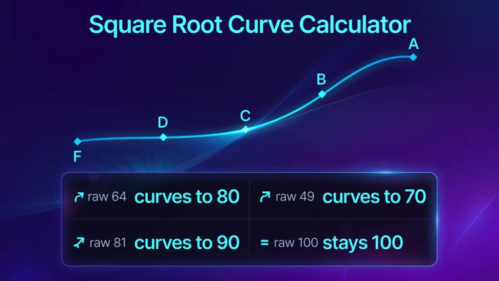
A square root curve calculator takes a raw test score out of 100 and applies the square root curve: curved score = 10 × √(raw score). A raw 64 becomes 80, a raw 49 becomes 70, and a raw 100 stays 100. Low scores gain the most, high scores gain the least, and no score ever goes down.
How do I use the Square Root Curve Calculator?
Enter your raw score in the single box at the top of the page. The raw score is the mark you actually earned on the test, out of 100, before any curve is applied. It can be a whole number such as 64, or a decimal such as 72.5 if your test gave partial marks. The tool accepts any number from 0 to 100.
Press the calculate button and four labelled boxes appear. The first box is the curved score, shown to two decimal places. The second box is the points gained, which is the curved score minus the raw score. The third box is the letter grade before the curve, and the fourth box is the letter grade after the curve. Both letter grades use the same scale, which the tool states plainly: A is 90 and above, B is 80 and above, C is 70 and above, D is 60 and above, and F is below 60. Under the boxes, a sentence repeats the result in words, so the change is readable at a glance: a raw 64 curves to 80.00, a gain of 16.00 points, moving the grade from D to B.
Below the boxes, the tool shows the full square root curve table for raw scores 0, 10, 20, 30, 40, 50, 60, 70, 80, 90 and 100. Each row shows the curved score, the points gained, and the letter grade before and after. The table is the same for every score you enter, because the curve is fixed: the same raw score always curves to the same value. Use it to read off the curve for a whole class without entering each score one at a time.
If an input is wrong, the tool shows a plain-language error and no results. A blank box is rejected because the tool needs a number to work with. A score below 0 is rejected because a test score cannot be negative. A score above 100 is rejected because the tool is built for scores out of 100 — if your test was out of a different total, turn the score into a percentage first: divide the marks earned by the total marks, then multiply by 100. To turn a raw score into a percentage, the percentage calculator does that step for you.
What does a worked example look like?
Start with the example every square root curve page uses, because it is the cleanest check of the formula. A raw score of 64. Take the square root of 64, which is 8, and multiply by 10: 8 × 10 = 80. The curved score is 80.00, a gain of 16.00 points. On the A 90+, B 80+, C 70+, D 60+, F below 60 scale, the grade moves from D to B — two letter grades from one curve. That is the size of change the square root curve is known for, and it is why teachers reach for it when a test has gone badly for most of the class.
A second example shows a larger gain on a lower score. A raw score of 49. The square root of 49 is 7, and 7 × 10 = 70. The curved score is 70.00, a gain of 21.00 points, and the grade moves from F to C. A student who failed the test outright now passes it with a C, because 49 is low enough on the curve to earn the biggest kind of boost. Compare that with the first example: a raw 64 gained 16 points, but a raw 49 gained 21. The lower score gained more, which is the whole point of the method.
A third example shows the other end of the scale. A raw score of 81. The square root of 81 is 9, and 9 × 10 = 90. The curved score is 90.00, a gain of 9.00 points, and the grade moves from B to A. A strong student still gains, but only 9 points against the 21 points a raw 49 gained. That shrinking gain is what makes the curve fair in the eyes of the teachers who use it: it lifts the bottom of the class much more than the top.
A fourth example shows a score that is not a perfect square, so the arithmetic needs a calculator rather than mental maths. A raw score of 55. The square root of 55 is 7.416198, and multiplying by 10 gives 74.16 to two decimal places. The curved score is 74.16, a gain of 19.16 points, and the grade moves from F to C. A raw 55 is only 5 points below the pass mark of 60, but the curve lifts it by more than 19 points, because 55 sits in the part of the curve where the boost is still large. That is the same effect as the 49 example, just without the tidy whole numbers.
Two edge cases complete the picture. A raw score of 100 curves to 100.00, a gain of 0.00 points, because the square root of 100 is 10 and 10 × 10 = 100. A perfect score has nowhere to go, and the curve leaves it exactly where it is. A raw score of 0 curves to 0.00, a gain of 0.00 points, because the square root of 0 is 0. The curve cannot create points from a blank paper: a student who scored nothing gains nothing, which is a limit worth knowing before anyone promises that a curve will rescue every score.
What is a square root curve?
A square root curve is a grading adjustment in which each raw score is replaced by 10 times its square root. The formula is curved score = 10 × √(raw score), and it applies to scores on a 0–100 scale. It is also called the Texas curve, after the state where it became widely used in schools and universities, and it is one of the standard methods for grading on a curve. The 10 in the formula is there to bring the result back onto the 0–100 scale: the square root of a number from 0 to 100 is a number from 0 to 10, so multiplying by 10 stretches it back to the full range.
The curve is a single fixed rule applied to every student in exactly the same way. There is no judgement call per student and no adjustment for how the class did as a whole. The same raw score always gives the same curved score, in every class and every subject. That consistency is part of its appeal: a student can check the curve for themselves, and a teacher can apply it to a whole class with one formula in a spreadsheet, =SQRT(A2)*10, filled down the column.
The key property of the curve is that it is non-linear. It does not add the same number of points to every score. It adds many points to low scores, fewer points to middle scores, and almost none to high scores. A raw 25 becomes 50, a gain of 25 points. A raw 36 becomes 60, a gain of 24 points. A raw 64 becomes 80, a gain of 16 points. A raw 81 becomes 90, a gain of 9 points. A raw 96 becomes 97.98, a gain of only 1.98 points. The gain falls steadily as the raw score rises, and it reaches zero at 100. That shape is why the curve is used when a test turns out harder than the teacher expected and most of the class has scored low: it repairs the bottom of the distribution without inflating the top.
The curve also has two guarantees built into the maths. First, it never lowers a score: every raw score from 0 to 100 curves to a value equal to or higher than itself, because the square root of a number between 0 and 100, multiplied by 10, is always at least that number. Second, it never changes the rank order of students: a higher raw score always gives a higher curved score, so the student who scored highest before the curve still scores highest after it. No two students swap places, and no student overtakes another because of the curve.
Why does the square root curve help low scores most?
The reason sits in the shape of the square root function itself. Square roots grow quickly at first and then slow down. The square root of 1 is 1, of 4 is 2, of 9 is 3, of 16 is 4, of 25 is 5, of 36 is 6, of 49 is 7, of 64 is 8, of 81 is 9, and of 100 is 10. Each step up the raw scale adds less and less to the square root. Going from a raw 1 to a raw 4 adds 1 to the square root, but going from a raw 81 to a raw 100 — a gap of 19 raw points — adds only 1 to the square root as well. Multiply by 10 and the same pattern holds for the curved scores: big gains at the bottom, small gains at the top.
Put numbers on it. A raw 10 curves to 31.62, a gain of 21.62 points. A raw 20 curves to 44.72, a gain of 24.72 points — a large gain, because 20 sits near the steepest part of the curve. A raw 30 curves to 54.77, a gain of 24.77 points, which is the largest gain of all the round-number scores. From there the gain falls: a raw 40 gains 23.25 points, a raw 50 gains 20.71, a raw 60 gains 17.46, a raw 70 gains 13.67, a raw 80 gains 9.44, a raw 90 gains 4.87, and a raw 100 gains nothing. The peak gain is around a raw 25 to 30, and it shrinks steadily from there to the top of the scale.
That shape is exactly what a teacher wants when a test has gone wrong for most of the class. If the average raw score is 55, the class is failing, and the teacher believes the test was too hard rather than the students too weak, the curve lifts the average student from 55 to 74.16 — from an F to a C — while lifting the best student from 90 to only 94.87. The class average moves a long way, the top of the class barely moves, and the gap between the strongest and weakest students shrinks. A student who scored 30 and a student who scored 90 were 60 points apart before the curve; after it they are 54.77 and 94.87, only 40.10 points apart. The curve compresses the spread, which is the other way of saying it narrows the differences between students.
That compression is also the curve’s main drawback, and it deserves a plain statement. When the top of the class is squeezed together, the curve stops telling strong students apart. A raw 90 and a raw 96 are 6 points apart before the curve and only 2.49 points apart after it (94.87 against 97.98). A raw 95 and a raw 100 are 5 points apart before the curve and 2.53 points apart after it. If a teacher needs to separate the best students — for a prize, a place on a team, or a grade boundary that matters — the square root curve blurs exactly the distinctions they need. It is a tool for lifting a class that has scored low, not for ranking students who have scored high.
What does the full square root curve table look like?
The table below is computed from the formula curved score = 10 × √(raw score), with every figure checked in Node. It shows the curved score, the points gained, and the letter grade before and after for each raw score from 0 to 100 in steps of 10. The tool on this page builds the same table live, so the figures here and the figures in the tool always agree.
| Raw score | Curved score | Points gained | Grade before | Grade after |
|---|---|---|---|---|
| 0 | 0.00 | +0.00 | F | F |
| 10 | 31.62 | +21.62 | F | F |
| 20 | 44.72 | +24.72 | F | F |
| 30 | 54.77 | +24.77 | F | F |
| 40 | 63.25 | +23.25 | F | D |
| 50 | 70.71 | +20.71 | F | C |
| 60 | 77.46 | +17.46 | D | C |
| 70 | 83.67 | +13.67 | C | B |
| 80 | 89.44 | +9.44 | B | B |
| 90 | 94.87 | +4.87 | A | A |
| 100 | 100.00 | +0.00 | A | A |
Three things in the table are worth reading closely. First, the grade changes happen at the bottom and the middle, not the top. A raw 40 moves from F to D, a raw 50 from F to C, a raw 60 from D to C, and a raw 70 from C to B. But a raw 80 stays a B and a raw 90 stays an A, because the curve cannot push them over the next boundary — a raw 80 would need a curved 90 to reach an A, and it reaches only 89.44. Second, the largest gain in the table is at raw 30, not at the lowest score: the gain rises from 21.62 at raw 10 to 24.77 at raw 30, then falls all the way to zero. Third, a raw 10 still fails after the curve — 31.62 is still an F — so the curve rescues students in the 30s, 40s and 50s, but not students who scored almost nothing.
The boundaries between letter grades fall on round raw scores, which makes the table easy to use without a calculator. A raw 36 curves to exactly 60.00, which is the D boundary. A raw 49 curves to exactly 70.00, the C boundary. A raw 64 curves to exactly 80.00, the B boundary. A raw 81 curves to exactly 90.00, the A boundary. Those four numbers — 36, 49, 64 and 81 — are the squares of 6, 7, 8 and 9, and they are the reason the worked examples on this page and on every other square root curve page use the same scores. They are also the numbers a student needs if they want to know what raw score earns each grade after the curve.
How do I work backwards: what raw score do I need?
The curve can be run in reverse. If you know the curved score you want, the raw score you need is the curved score divided by 10, squared: raw score = (curved score ÷ 10)². That is the inverse of the curve formula, and it answers the question students actually ask: what do I need to score on the test to end up with the grade I want?
The four grade boundaries give the cleanest answers. To finish with a curved 90, an A, you need a raw 81, because (90 ÷ 10)² = 81. To finish with a curved 80, a B, you need a raw 64, because (80 ÷ 10)² = 64. To finish with a curved 70, a C, you need a raw 49, because (70 ÷ 10)² = 49. To finish with a curved 60, a D and a pass, you need a raw 36, because (60 ÷ 10)² = 36. Those are the same four numbers as the table above, read in the other direction.
The in-between targets are less tidy but just as useful. To finish with a curved 85, a solid B, you need a raw 72.25, because (85 ÷ 10)² = 72.25. To finish with a curved 95, a high A, you need a raw 90.25, because (95 ÷ 10)² = 90.25. That last figure carries a warning of its own: the difference between a curved 90 and a curved 95 is 5 points, but the raw difference is 9.25 points (81 against 90.25). At the top of the scale, each extra curved point costs more and more raw points, because the curve is nearly flat there. A student aiming for a curved 95 from a raw 90 gains only 4.87 points from the curve, and would need to earn almost all of the extra marks themselves.
That is the practical use of the inverse formula. Before a test, a student who knows their teacher curves with the square root method can work out the raw score that earns the grade they need, and aim at that number rather than at the grade boundary itself. A student who needs a C needs a raw 49, not a raw 70. A student who needs a B needs a raw 64, not a raw 80. The gap between the two numbers is the help the curve gives, and knowing it in advance changes how much of the test a student needs to get right.
How does the square root curve compare with flat points and a bell curve?
Teachers have more than one way to curve grades, and the square root curve is one choice among several. The comparison that matters most is with the flat-points curve, because it is the simplest method and the one most teachers try first. A flat-points curve adds the same number of points to every score: curved score = raw score + a fixed number, capped at 100. A +10 flat curve turns a raw 25 into 35, a raw 64 into 74, a raw 81 into 91, and a raw 90 into 100.
Set the two methods side by side at the same raw scores and the difference is plain. At a raw 25, the square root curve gives 50.00, a gain of 25 points, while a +10 flat curve gives 35, a gain of 10. At a raw 64, the square root curve gives 80.00, a gain of 16, while the flat curve gives 74, a gain of 10. At a raw 81, the square root curve gives 90.00, a gain of 9, while the flat curve gives 91, a gain of 10 — here the flat curve gives slightly more. At a raw 90, the square root curve gives 94.87, a gain of 4.87, while the flat curve gives 100, a gain of 10. At a raw 96, the square root curve gives 97.98, a gain of 1.98, while the flat curve gives 100, a gain of 4 after the cap.
The pattern is clear. Below a raw 81, the square root curve gives more than a +10 flat curve. Above a raw 81, the flat curve gives more. The two methods cross at a raw 81, where the square root curve gives exactly 90 and the flat curve gives exactly 91 — close enough that the difference is one point. The square root curve is the better choice when the problem is at the bottom of the class: many low scores that need a large lift. The flat curve is the better choice when the problem is spread evenly, or when the teacher wants every student to gain the same amount and keep the gaps between students exactly as they were. A flat curve preserves every gap: a 10-point gap between two students stays a 10-point gap. The square root curve shrinks every gap, which is a help when the gaps were caused by a test that was too hard, and a problem when the gaps were real differences in how much students knew.
The bell curve is a different kind of method again. Instead of applying a fixed formula to each score on its own, it looks at the whole class: it works out the class average and how spread out the scores are, then moves each score to a new position based on how far it sits from the average. A student at the class average stays near the average, a student one step above it moves up by a set amount, and a student one step below it moves down by the same amount. That last point is the key difference. A bell curve can lower a score: a student who scored above the class average on a test where the average was high can end up with a lower grade after the curve. The square root curve never lowers a score, and neither does a flat-points curve. A bell curve also needs the whole class’s scores to work, while the square root curve needs only one student’s score. For a student checking their own grade, or a teacher curving one paper, the square root curve is the method that works with a single number.
A fourth method is the top-score method: add the gap between the highest score and 100 to every student. If the best score in the class was 85, everyone gains 15 points. That method is a flat curve whose size depends on the best student, so it shares the flat curve’s even-handedness and its weakness — it gives the same lift to a student who scored 30 as to a student who scored 85. The square root curve is the only common method that gives a bigger lift to the students who scored lowest, and that is why it is the method teachers choose when the low scores are the problem.
When do teachers use a square root curve?
Teachers use a square root curve when a test turns out harder than intended and the raw scores do not reflect what the class actually learned. The usual signs are a class average far below the pass mark, a large number of failing grades on a test the teacher expected most students to pass, or a single question that turned out to be unclear or wrong and dragged many scores down. In those cases the teacher’s judgement is that the test, not the students, was at fault, and the curve is the correction. It is used most often in maths, physics, chemistry and other STEM subjects, and in AP classes, where tests are deliberately hard and a raw score in the 60s can represent solid understanding.
The curve is applied after the test is marked, to the whole class at once, and it is announced rather than hidden. A teacher who curves will usually tell the class the method they used, because the curve changes the meaning of the grade and students need to know how their final mark was reached. The curve is also a one-off decision for one test, not a standing policy for the whole course. A teacher who curves every test with the same method is effectively redefining the grade scale, and the grades stop meaning what the syllabus says they mean.
There are times when a teacher will not use it. If the class average is already reasonable, there is nothing to fix and a curve would inflate grades for no reason. If only a few students scored low while most did well, the problem is with those students’ preparation, not with the test, and curving the whole class would reward the students who did not prepare. If the grades matter for ranking — a scholarship, a place on a competitive programme, a prize — the compression at the top of the curve blurs the differences the ranking needs. And if the test itself was fair and the scores are an honest picture of what students knew, many teachers will leave the scores alone, because the grades are meant to say how much was learned, not how kind the marking was.
Students cannot claim a curve. It is the teacher’s decision, made after marking, and it applies to the whole class or to nobody. A student who asks for a square root curve on their own paper is asking the teacher to change the rules for one person, which no fair marking system allows. What a student can do is use this calculator to see what their grade would be if the teacher does curve, and to work out, from the inverse formula, what raw score they need for the grade they want.
What are the limits of a square root curve?
The first limit is the one already covered: the curve compresses the top end. It cannot separate strong students, and it gives a student who scored 96 only 1.98 extra points while giving a student who scored 30 an extra 24.77. If the purpose of the grades is to tell strong students apart, the curve works against that purpose. A teacher who needs to distinguish an A student from an A+ student should not use it.
The second limit is that the curve cannot fix a bad test. It can lift scores, but it cannot repair questions that were wrong, unclear or off-syllabus, and it cannot tell the teacher which questions caused the problem. A test where half the class failed because two questions were misworded needs those questions thrown out or re-marked, not a curve applied to the whole paper. The curve treats every low score the same way, whether the student misunderstood the material or the question itself was at fault, and that bluntness is a limit, not a feature.
The third limit is that the curve cannot create points from nothing. A raw 0 stays 0, a raw 1 becomes 10.00, and a raw 10 becomes only 31.62 — still an F. Students who scored almost nothing gain little in absolute terms, because the curve multiplies what is there rather than adding a fixed amount. A flat-points curve would give a raw 10 the same 10 points it gives everyone else; the square root curve gives it 21.62, which is more, but still leaves the student failing. No curve can rescue a paper with almost nothing right on it.
The fourth limit is that the curve changes what the grade means. A curved 80 is not the same as a raw 80: one student earned 80% of the marks, the other earned 64% and was lifted to 80 by the formula. If the grade is later used to judge whether a student is ready for the next course, or to compare students from different classes where one teacher curved and the other did not, the curved grade overstates what the student demonstrated. That is why teachers who curve usually note it on the record, and why a curved grade should be read as a grade after adjustment, not as a raw mark.
The fifth limit is the grade scale itself. This tool uses A 90+, B 80+, C 70+, D 60+, F below 60, which is the most common scale, but schools and universities use other scales, and a curved 89.44 is a B on this scale and an A on a scale where A starts at 89. The curve does not set the grade boundaries; the school does. A student should check their own school’s scale before reading a letter grade off this tool, and a teacher should apply their own scale to the curved scores rather than taking the tool’s letters as final.
How is this different from a weighted grade calculator?
A weighted grade calculator and a square root curve calculator answer different questions, and the two are easy to confuse because both deal with grades. The live grade calculator with weights takes the scores a student has earned on assignments, tests and homework, together with the weight each one carries in the final grade, and works out the weighted average. If homework is worth 20% and the final exam is worth 40%, the tool combines them in those proportions and returns the average the student has earned so far. It never changes a score. A test marked 64 stays 64, and the average is built from the marks as they are.
This tool does the opposite job. It takes one raw score and changes it, applying the square root formula to produce a curved score that is higher than the raw score. It has no weights, no list of assignments, and no average. It answers the question “what would this score become if the teacher curved it?” while the weighted calculator answers “what is my average across everything I have done so far?” A student who wants to know their course average uses the weighted calculator. A student who wants to know what a single curved test score would be uses this one. The two tools sit side by side in the calculators category, and they are used together when a teacher curves a test and then folds the curved score into a weighted average — curve first, then weight.
The same distinction applies to the GPA calculator, which turns letter grades into a grade point average. A GPA calculator takes grades that already exist and combines them into one number; it does not change any grade, and it does not apply a curve. If a curved score changes a letter grade from D to B, the GPA calculator will give a higher GPA — but only because the grade fed into it changed. The curve is the step that changes the grade, and this tool is the step that works the curve out.
How can I check the tool against a known score?
The simplest check uses the first verified test. Enter a raw score of 64. The tool should show a curved score of 80.00, points gained of +16.00, a letter grade before the curve of D (64.00), and a letter grade after the curve of B (80.00). The note under the boxes should read: “A raw score of 64.00 curves to 80.00, a gain of 16.00 points, moving the grade from D to B.” Every box should match. If any box differs, an entered value differs from the test, and the error is in the input rather than in the tool.
A second check uses the largest gain in the low range. Enter a raw score of 49. The tool should show a curved score of 70.00, points gained of +21.00, a letter grade before the curve of F (49.00), and a letter grade after the curve of C (70.00). A third check uses a score that is not a perfect square. Enter a raw score of 55. The tool should show a curved score of 74.16, points gained of +19.16, a letter grade before the curve of F (55.00), and a letter grade after the curve of C (74.16). A fourth check uses the top of the scale: enter a raw score of 81 and the tool should show a curved score of 90.00, points gained of +9.00, a letter grade before the curve of B (81.00), and a letter grade after the curve of A (90.00).
A fifth check uses the table. Enter any raw score, then read the table row for a raw 30: it should show a curved score of 54.77, points gained of +24.77, a grade before of F and a grade after of F. The row for a raw 50 should show a curved score of 70.71, points gained of +20.71, a grade before of F and a grade after of C. The row for a raw 90 should show a curved score of 94.87, points gained of +4.87, and a grade of A before and after.
A sixth check tests the edges. Enter a raw score of 100 and the tool should show a curved score of 100.00, points gained of +0.00, and a grade of A before and after. Enter a raw score of 0 and the tool should show a curved score of 0.00, points gained of +0.00, and a grade of F before and after. Enter 105 and the tool should show the error “The raw score cannot be above 100. Enter your score out of 100.” with no results. Enter −5 and it should show “The raw score cannot be below 0.” with no results. Leave the box blank and it should show “Please enter your raw score (a number from 0 to 100).” with no results.
The formula behind the tool is the standard square root curve formula, as set out in the step-by-step explanation on NumbrWiz, which gives the formula as curved score = √(raw ÷ max) × max and works the 64 to 80 example through its three steps, and in the grade-curve guide on TeacherCalculator, which gives the formula as curved score = √(raw score) × 10 and works the same 64 to 80 example, with 36 to 60 and 81 to 90 alongside it. The comparison with flat-points and bell-curve methods follows the method-by-method explanations in the All In One Generators guide to curving grades, which lists the square root, flat-points, top-score and bell-curve methods with their formulas and when each fits. More tools in the same collection are in the calculators category.
Frequently asked questions
What is a square root curve calculator?
It is a tool that applies the square root curve to a raw test score: curved score = 10 × √(raw score), for scores on a 0–100 scale. A raw 64 becomes 80, a raw 49 becomes 70, and a raw 100 stays 100. Low scores gain the most points and high scores gain the least, and no score ever goes down. Enter your raw score and this calculator shows the curved score, the points gained, and the letter grade before and after.
How do you calculate a square root curve?
Take the square root of the raw score and multiply by 10. For a raw 64, the square root of 64 is 8, and 8 × 10 = 80, so the curved score is 80. For a raw 49, the square root is 7, and 7 × 10 = 70. For a raw score that is not a perfect square, use a calculator: the square root of 55 is 7.416198, and multiplying by 10 gives a curved score of 74.16. The general form for a test out of a different total is curved score = √(raw ÷ max) × max.
Why does a square root curve help low scores more than high scores?
Because square roots grow quickly at first and then slow down. Going from a raw 1 to a raw 4 adds 1 to the square root, but going from a raw 81 to a raw 100 — a gap of 19 raw points — also adds only 1. So a raw 25 gains 25 points to reach 50, a raw 64 gains 16 points to reach 80, a raw 81 gains 9 points to reach 90, and a raw 96 gains only 1.98 points to reach 97.98. The gain is largest around a raw 25 to 30 and falls steadily to zero at 100.
Can a square root curve lower my grade?
No. The square root curve never lowers a score: every raw score from 0 to 100 curves to a value equal to or higher than itself. It also never changes the rank order of students, because a higher raw score always gives a higher curved score. A raw 100 stays 100 and a raw 0 stays 0, so the curve cannot raise a perfect score or create points from a blank paper. Other methods can lower a score — a bell curve can move a score down — but the square root curve cannot.
What raw score do I need for a curved 90?
You need a raw 81, because the curve runs in reverse as raw score = (curved score ÷ 10)², and (90 ÷ 10)² = 81. The same rule gives the other grade boundaries: a curved 80 needs a raw 64, a curved 70 needs a raw 49, and a curved 60 needs a raw 36. For a curved 85 you need a raw 72.25, and for a curved 95 you need a raw 90.25. At the top of the scale each extra curved point costs more raw points, because the curve is nearly flat there.
Is a square root curve the same as adding points to every grade?
No. Adding the same number of points to every score — a flat-points curve — gives every student the same lift and keeps the gaps between students exactly as they were. The square root curve gives a bigger lift to low scores and a smaller lift to high scores, and it shrinks the gaps between students. Below a raw 81 the square root curve gives more than a +10 flat curve (a raw 64 becomes 80 instead of 74), and above a raw 81 the flat curve gives more (a raw 90 becomes 100 instead of 94.87). Teachers choose the square root curve when the low scores are the problem.